The Very Tiny Constraint Solver
Charles Prud'homme, March 2024IMT Atlantique, LS2N, TASC
< press [N] / [P] to go the next / previous slide >
In this presentation, we are going to code from scratch a minimalist constraint solver.
The aim is nothing but understanding the internal mechanics.
Spoiler alerts
There are already plenty of great open source constraint solvers:
choco-solver🐙, or-tools, gecode, ACE, JaCoP, Mistral, Chuffed, …
🐙 My favourite.... but I am biasedAnd several excellent constraint modeling languages:
MiniZinc, XCSP3 / PyCSP3, CPMpy, …
So basically here we are not going to reinvent the wheel or break the paradigm but just
understand by doing
A little bit of theory
We are talking about Constraint Satisfaction Problem .
A CSP $\mathcal{P}$ is a triple $\left<\mathcal{X},\mathcal{D},\mathcal{C}\right>$ where:
- $\mathcal{X} = \{X_1, \ldots, X_n\}$ is a set of variables,
- $\mathcal{D}$ is a function associating a domain to each variable,
- $\mathcal{C}$ is a set of constraints.
It can be turn into a COP quite easily
Let’s consider the following CSP $\mathcal{P}$:
- $\mathcal{X} = \{X_1, X_2, X_3\}$
- $\mathcal{D} = \{D(X_1)=D(X_2)=[1,2], D(X_3)=[1,3]\}$
- $\mathcal{C} = \{X_1\leq X_2,X_2\leq X_3,AtMost(1,[X_1, X_2, X_3],2)\}$
A constraint defines a relation between variables.
It is said to be satisfied if :
- its variables are instantiated to a single value*
- and the relation holds
In $\mathcal{P}$, the constraint $AtMost(1,[X_1, X_2, X_3],2)$ holds iff at most 1 variable among $X_1, X_2, X_3$ is assigned to the value 2.
- $(1,1,1)$ and $(1,2,3)$ satisfy the constraint,
- $(2,2,1)$ does not.
The constraints can be defined in intension or in extension .
For $X_1$, $X_2$ on domains $\{1,2\}$:
- intension:
- expression in a higher level language
- e.g., $X_1+X_2\le3$
- extension:
- allowed combinations
- e.g., ${(1,1),(1,2),(2,1)}$
Less formally
What we know about a variable is that :
- it takes its values from a domain
*, e.g.,
{1,2,3,5}, - it is linked to other variables using constraints ,
- and it must be instantiated in a solution .
On the other hand, a constraint :
- defines a contract between its variables,
- must be satisfied in every solutions,
- and is more than just a checker.
Choose your favourite programming language
(I chose Python)
and let’s get started
Variables and domains
Let’s make it simple
A variable will be referenced by a key, its name.
A domain will be associated to it.
Beware: each value can appear only once.
A dictionary and sets will do :
>>🥛<<
This clickable logo indicates that a workshop is available at Caseine
A dictionary and sets will do :
variables = {"x1": {1, 2, 3},
             "x2": {1, 2, 3}}
and that’s enough.
🚀 Possible improvements
- Creating a variable object
- Effective domain representation (e.g., bitset)
- Introducing variable views (e.g., $y = a.x + b$)
- Other types of variable (e.g., Boolean, set, graph)
Constraints
$X_1 < X_2$
Such a constraint will take two variables as argument and makes sure that the former one takes a value less than the latter one in any solution.
$(1,2)$ and $(2,5)$ satisfy the constraint,
$(2,2)$ and $(5,3)$ do not.
We will first create a class to declare the behaviour of this constraint:
class LessThan:
    def __init__(self, v1, v2):
        self.v1 = v1
        self.v2 = v2
We can impose that $X_1$ is strictly less than $X_2$:
variables = {"x1": {1, 2, 3},
             "x2": {1, 2, 3}}
c1 = LessThan("x1", "x2") # means that x1 < x2 should hold
What can such a constraint do?
In CP, we remove
The basic behaviour of a constraint is to remove from the variable domain those values that cannot be extended to any solution
(according to its own contract)
We will create an empty function called filter as follow:
def filter(self,variables):
	pass
The 2 rules of $X_1 < X_2$
1. removing from $X_1$ values greater or equal to the largest value in $X_2$,
2. removing from $X_2$ values smaller or equal to the smallest value in $X_1$.
Otherwise, in both cases, we could break the contract established between the 2 variables.
$X_1 = \{1,2,3,4\}$, $X_2 = \{1,2,3,4\}$ and $X_1 < X_2$
Then
- 4 is removed from $X_1$
- 1 is removed from $X_2$
In other words:
- $max(X_2)$ and larger are removed from $X_1$
- $min(X_1)$ and smaller are removed from $X_2$
Deal with dead ends
We can tell that the constraint should return :
True: if some values were filteredFalse: if a domain becomes emptyNone: if nothing was filtered
LessThan filtering algorithm
class LessThan:
    def __init__(self, v1, v2):
        self.v1 = v1
        self.v2 = v2

    def filter(self, variables):
        """
        Filter the domain of the variables declared in 'vars'.
        The method directly modifies the entries of 'vars'.
        It returns True if some values were filtered,
        False if a domain becomes empty,
        None otherwise.
        """
        pass
>>🥛<<
LessThan filtering algorithm
def filter(self, variables):
    cd1 = variables[self.v1] # get current domain of "x1"
    cd2 = variables[self.v2] # get current domain of "x2"
    # filtering according to the 1st rule
    nd1 = {v for v in cd1 if v < max(cd2)}
    if len(nd1) == 0: # "x1" becomes empty...
        return False
    # filtering according to the 2nd rule
    nd2 = {v for v in cd2 if v > min(cd1)}
    if len(nd2) == 0: # "x2" becomes empty...
        return False
    variables[self.v1] = nd1 # update the domain of "x1"
    variables[self.v2] = nd2 # update the domain of "x2"
    modif = cd1 > nd1 or cd2 > nd2 # reduction of a domain
    return modif or None
Does that work?
# declare a CSP
variables = {"x1": {1, 2, 3},
             "x2": {1, 2, 3}}
c1 = LessThan("x1", "x2")
# call the filtering algorithm
modif = c1.filter(variables)
# check everything works fine
assert variables["x1"] == {1, 2}
assert variables["x2"] == {2, 3}
assert modif == True
Yes, it does !
Filtering is not enough
It didn’t build a solution
although all impossible values were removed
It seems that we need to dive into the
search space 🤿
in a DFS way.
Adapting the DFS
- If all variables are fixed, stop the search
- If inconsistency detected, then backtrack
- Expand the tree by making a decision$^*$

Backtracking
For this, we need to retrieve the state of the domains before a decision is applied.And therefore it must have been registered beforehand.
And we must be able to rebut a decision.
Search strategy
How to select the next decision to apply?
select an uninstantiated variable
pick a value in its domain (e.g., the lower bound)
A recursive approach should simplify our task
Let’s break down the needs into 4 functions.
def make_decision(variables):
    pass

def copy_domains(variables):
    pass

def apply_decision(variables, var, val, apply, constraint):
    pass

def dfs(variables, constraint):
    pass
>>🥛<<
def make_decision(variables):
    var, dom = next(
        filter(lambda x: len(x[1]) > 1, variables.items()),
        (None, None))
    if var is not None:
        # if true, returns the decision
        return (var, min(dom))
    else:
        # otherwise, all variables are instantiated
        return None
def copy_domains(variables):
    # returns a deep copy of the dictionnary
    return {var: dom.copy() for var, dom in variables.items()}
def apply_decision(variables, var, val, apply, constraint):
  # copy the domains
  c_variables = copy_domains(variables)
  # applies the decision or rebuts is
  c_variables[var] = {x for x in c_variables[var] \
                      if apply is (x == val)}
  # explore the sub-branch
  return dfs(c_variables, constraint)
def dfs(variables, constraint):
  constraint.filter(variables)
  dec = make_decision(variables)
  if dec is None:
      print(variables)  # prints the solution
      return 1
  else:
      var, val = dec
      n = apply_decision(variables, var, val, True, constraint)
      n += apply_decision(variables, var, val, False, constraint)
  return n
variables = {"x1": {1, 2, 3},
             "x2": {1, 2, 3}}
c1 = LessThan("x1", "x2")

print("There are", dfs(variables, c1), "solutions")
should output:
{'x1': {1}, 'x2': {2}}
{'x1': {1}, 'x2': {3}}
{'x1': {2}, 'x2': {3}}
There are 3 solutions
We did it !
Well almost, but still you can pat yourself back !
🚀 Managing backups
📄“Comparing trailing and copying for constraint programming”, C. Schulte, ICLP'99.
- Copying: An identical copy of S is created before S is changed.
- Trailing: Changes to S are recorded such that they can be undone later.
- Recomputation: If needed, S is recomputed from scratch.
- Adaptive recomputation: Compromise between Copying and Recomputation.
🚀 Making decisions
- Dynamic criteria for variable selection
- And value selection (min, max, mid, rnd)
- Different operators ($=, \neq, \leq, \geq$)
- Depth-first, limited-discrepancy, large neighborhood
Back to work
deal with failures
Let’s fix the code
def dfs(variables, constraint):
    # manage filtering failure
>>🥛<<
Let’s fix the code
def dfs(variables, constraint):
    if constraint.filter(variables) is False:
        return 0
    var, val = make_decision(variables)
    if var is None:
        print(variables)
        return 1
    else:
        n = propagate(variables, var, val, True, constraint)
        n += propagate(variables, var, val, False, constraint)
        return n
None and True will be used later.
This code
variables = {"x1": {3, 4},
             "x2": {2, 3}}
c1 = LessThan("x1", "x2")

print("There are", dfs(variables, c1), "solutions")
outputs:
There are 0 solutions
🚀 Possible improvements
- Explaining failures (LCG)
- Adapting the research strategy:
- dom/wdeg, pick-on-dom, ABS, etc
- last conflict, conflict ordering search
Many constraints
of the same type
variables = {"x1": {1, 2, 3},
             "x2": {1, 2, 3},
             "x3": {1, 2, 3}}
c1 = LessThan("x1", "x2")
c2 = LessThan("x2", "x3")
We need to adapt the dfs(_,_) function:
def dfs(variables, constraints):
    # if constraint.filter(variables) is False:
    if not fix_point(variables, constraints):
        return 0 # at least one constraint is not satisfied
    # ...
and ensure that a fix point is reached.
Fixpoint reasoning
Iteratively applying constraint propagation until no more improvements are possible or a failure is detected.
So, as long as a constraint filters values, all the other ones must be checked.
🚀 This could be refined.
| step | x1 | x2 | x3 | To check | Consistent |
|---|---|---|---|---|---|
| 0 | [1,3] | [1,3] | [1,3] | {c1,c2} | {} |
| 1 | [1,2] | [2,3] | - | {c1,c2} | {} |
| {c2} | {c1} | ||||
| 2 | - | [2,2] | [3,3] | {c2} | {c1} |
| {c1} | {c2} | ||||
| 3 | [1,1] | - | - | {c1} | {c2} |
| {c2} | {c1} | ||||
| 4 | - | - | - | {c2} | {c1} |
| {} | {c1, c2} |
We will create a method to iterate on the constraints:
def fix_point(variables, constraints):
    """Reach a fix point.
    If a failure is raised, returns False,
    otherwise guarantees that all events are propagated.
    """
>>🥛<<
def fix_point(variables, constraints):
    while True:
        fltrs = False
        for c in constraints:
            flt = c.filter(variables)
            if flt is False: # in case of failure
                return False
            elif flt is True: # in case of filtering
                fltrs |= True # keep on looping
        if not fltrs : # to break the while-loop
            return True
variables = {"x1": {1, 2, 3},
             "x2": {1, 2, 3},
             "x3": {1, 2, 3}}
c1 = LessThan("x1", "x2")
c2 = LessThan("x2", "x3")
fix_point(variables, {c1, c2})
print(variables)
outputs:
{'x1': [1], 'x2': [2], 'x3': [3]}
🚀 Propagation engine
- Event-based reasoning, advisors, watch literals
- Scheduling and propagating
- Variable-oriented or Constraint-oriented
- Iterating on constraints by considering their complexity
Many constraints
of the different type
Adding the constraint
$X_1\neq X_2 + c$
where $c$ is a constant
should be quite easy
It requires to define the filter function.
The 2 rules of $X_1\neq X_2 + c$
1. if $X_2$ is instantied to $v_2$, then $v_2+c$ must be removed from $X_1$ values,
2. if $X_1$ is instantied to $v_1$, then $v_1-c$ must be removed from $X_2$ values.
Let’s fix the code
  class NotEqual:
      def __init__(self, v1, v2, c=0):
          pass

      def filter(self, vars):
          pass
>>🥛<<
The NotEqual class
class NotEqual:
    def __init__(self, v1, v2, c=0):
        self.v1 = v1
        self.v2 = v2
        self.c = c

    def filter(self, vars):
      size = len(vars[self.v1]) + len(vars[self.v2])
      if len(vars[self.v2]) == 1:
          f = min(vars[self.v2]) + self.c
          nd1 = {v for v in vars[self.v1] if v != f}
          if len(nd1) == 0:
            return False
          vars[self.v1] = nd1
      if len(vars[self.v1]) == 1:
          f = min(vars[self.v1]) - self.c
          nd2 = {v for v in vars[self.v2] if v != f}
          if len(nd2) == 0:
            return False
          vars[self.v2] = nd2
      modif = size > len(vars[self.v1]) + len(vars[self.v2])
      return modif or None
🚀 Constraints
- Different level of inconsistency
- Global reasoning vs decomposition
- Explain domain modifications
- Reification, entailment, …
Now, we are able to
solve a basic problem
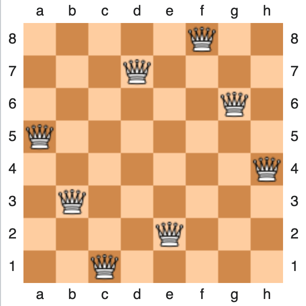
The 8 queens puzzle
The eight queens puzzle is the problem of placing eight chess queens on an 8×8 chessboard so that no two queens threaten each other; thus, a solution requires that no two queens share the same row, column, or diagonal.
A first idea is to indicate by a Boolean variable if a cell is occupied by a queen or not.
But we wouldn’t be able to use our constraints.
Also, it is very MILP-like or SAT-like.
A more CP way to model it
A variable per column.
Each domain encodes the row where the queen is set.
Four groups of inequality constraints are posed:
- no two queens share the same row
- no two queens share the same column (➡️ handled by the model 🤘)
- no two queens share the same upward diagonal
- no two queens share the same downward diagonal
>>🥛<<
6 Queens puzzle in Python
import model as m

n = 8
vs = {}
for i in range(1, n + 1):
    vs["x" + str(i)] = {k for k in range(1, n + 1)}

cs = []
for i in range(1, n):
    for j in range(i + 1, n + 1):
        cs.append(m.NotEqual("x" + str(i), "x" + str(j)))
        cs.append(m.NotEqual("x" + str(i), "x" + str(j), c=(j - i)))
        cs.append(m.NotEqual("x" + str(i), "x" + str(j), c=-(j - i)))

# mirror symm. breaking
vs["cst"] = {int(n / 2) + 1}
cs.append(m.LessThan("x1", "cst"))

# search for all solutions
sols = []
m.dfs(vs, cs, sols, nos=0)
print(len(sols), "solution(s) found")
print(sols)
46 solutions
46 solution(s) found
[[1, 5, 8, 6, 3, 7, 2, 4, 5], ..., [4, 8, 5, 3, 1, 7, 2, 6, 5]]
There are 92 solutions without the (simple) symmetry breaking constraint, 46 otherwise.
We did it 🍾
We build a minimalist CP solver :
- based on integer variables,
- using two different types of constraints,
- each equipped with a filtering algorithm,
- exploring the search space in DFS way.
And we were able to enumerate solutions on a puzzle !
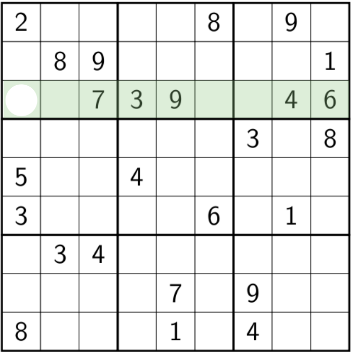
Analogy with Sudoku
We reached the Sudoku point
When trying to explain how constraint programming works, it is common to draw a parallel with sudoku.
At modelling step
-
One must write a value in $[1,9]$ in each cell
- ➡️ a variable and a domain
-
Such that each digit is used exactly once per row , per column and per square
- ➡️ sets of $\neq$ constraints
At solving step
Local reasonning
Filtering
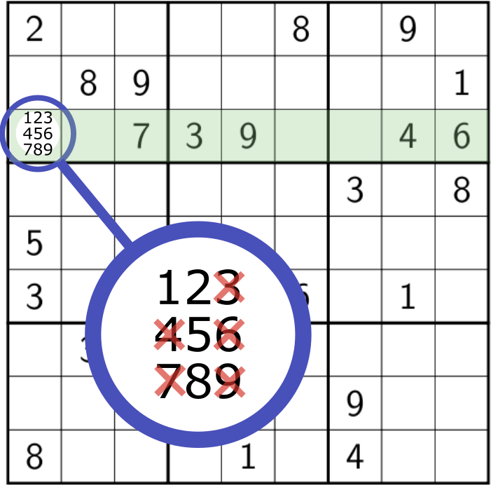
Propagation
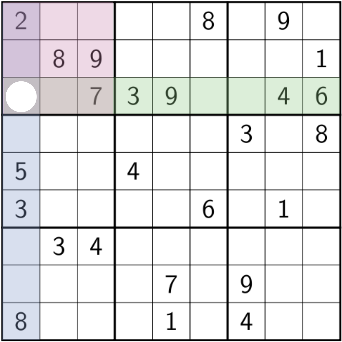
Search
On devil sudoku, one has to make assumptions.
And validate them by propagation.
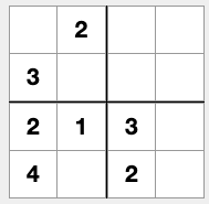
A 4x4 sudoku example
import model as m

n = 4
variables = {}
for i in range(1, n + 1):
    for j in range(1, n + 1):
        variables["x" + str(i) + str(j)] = {k for k in range(1, n + 1)}
# fix values
variables["x12"] = [2]
variables["x21"] = [3]
variables["x31"] = [2]
variables["x32"] = [1]
variables["x33"] = [3]
variables["x41"] = [4]
variables["x43"] = [2]

zones = []
# rows
zones.append(["x11", "x12", "x13", "x14"])
zones.append(["x21", "x22", "x23", "x24"])
zones.append(["x31", "x32", "x33", "x34"])
zones.append(["x41", "x42", "x43", "x44"])
# columns
zones.append(["x11", "x21", "x31", "x41"])
zones.append(["x12", "x22", "x32", "x42"])
zones.append(["x13", "x23", "x33", "x43"])
zones.append(["x14", "x24", "x34", "x44"])
# square
zones.append(["x11", "x12", "x21", "x22"])
zones.append(["x13", "x14", "x23", "x24"])
zones.append(["x31", "x32", "x41", "x42"])
zones.append(["x33", "x34", "x43", "x44"])

cs = []
for z in zones:
    for j in range(0, n):
        for k in range(j + 1, n):
            cs.append(NotEqual(z[j], z[k]))

sols = []
m.dfs(variables, cs, sols, nos=0)
print(len(sols), "solution(s) found")
u_sol = sols[0]
for i in range(4):
		print(u_sol[i * 4:i * 4 + 4])
1 solution
1 solution(s) found
[1, 2, 4, 3]
[3, 4, 1, 2]
[2, 1, 3, 4]
[4, 3, 2, 1]
The value of CP lies
in the constraints
We only saw two basic binary constraints.
But there are hundreds of them.
Why are there so many of them?
Is it not possible to do with less?
Indeed, MILP and SAT are doing very well with one type of constraint !
Two main reasons
- Modeling : stronger expressive power
- Solving : increased filter quality
At the modeling stage
- each constraint is semantically defined
- which also indicates the contract it guarantees
Examples
| Name | Purpose |
|---|---|
alldifferent |
enforces all variables in its scope to take distinct values |
increasing |
the variables in its scope are increasing |
maximum |
a variable is the maximum value of a collection of variables |
| … | |
Others are less obvious 😇
subgraph_isomorphism, path, diffn, geost, …
but are documented
At the modeling stage (2/2)
- A CSP model is a conjunction of constraints
- The model can be very compact
- It is easy to understand and modify a model
Recall that there are modelling languages to do this
At solving stage
But it is rather here that one can measure the interest of the constraints
A constraint captures a sub-problem
and provides an efficient way to deal with it
thanks to an adapted filtering algorithm
On one example
$\bigwedge_{X_i,X_j \in X, i\neq j} X_i \neq X_j$
-vs-
$\texttt{allDifferent}(X)$
Both version find the same solutions
but the 2nd filters more
With binary constraints

What can be deduced?
Nothing until a variable is set
With a global constraint
Rely on graph theory…
With a global constraint

pair variables and values in a bipartite graph…
With a global constraint

find maximum cardinality matchings…
With a global constraint

remove values which belong to none of them.
Summary
| $\bigwedge_{x_i,x_j \in X, i\neq j} x_i \neq x_j$ | $\texttt{allDifferent}(X)$ | |
|---|---|---|
| #cstrs | $\frac{\vert X \vert \times \vert X\vert -1}{2}$ | 1 |
| Filtering | weak and late | arc-consistency in polynomial time and space |
| Algorithm | straightforward | tricky* |
*: but already done for you in libraries
Remarks about global constraints
Many model highly combinatorial problems
It is likely that:
- arc-consistency is not reached (i.e., weaker filtering)
- filtering is complex to achieve
Their expressive power remains strong
Improvements
that we do not develop
At the modelling level
- Other kinds of variables
- Other constraints or way to express rules
- Search space exploration
- Black-box strategies,
- Restarting,
- Alternatives to DFS
At the solving step
- Refine the way constraints are propagated
- Fine response of propagators to variables’ changes
- Restore by copy or trail
- Conflict-driven Clause-learning
- …
And so many other things !
Thank you
Q?