The connector problem

Description from Bondy, J. and Murty, U. (1976) Graph Theory with Applications. MacMillan, London.

A railway network connecting a number of towns is to be set up. Given the cost $c_{ij}$ of constructing a direct link between towns $v_i$ and $v_j$, design such a network to mininlise the total cost of construction. This is known as the connector problem. By regarding each town as a vertex in a weighted graph with weights $w(v_ivj) = c_{ij}$, it is clear that this problem is just that of finding, in a weighted graph $G$, a connected spanning subgraph of minimum weight. Moreover, since the weights represent costs, they are certainly non-negative, and we may therefore assume that such a minimum-weight spanning subgraph is a spanning tree $T$ of $G$. A minimum-weight spanning tree of a weighted graph will be called an optimal tree.

Definition (Minimum Spanning Tree): A minimum weight spanning tree is a subset of the edges of a connected, edge-weighted undirected graph that connects all the vertices together, without any cycles and with the minimum possible total edge weight.

As an example, we can consider the problem of finding airline network where the objective is to reach all given towns and the cost is relative to the distance between them.

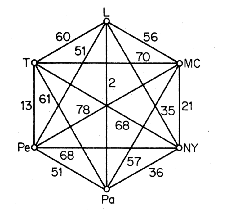
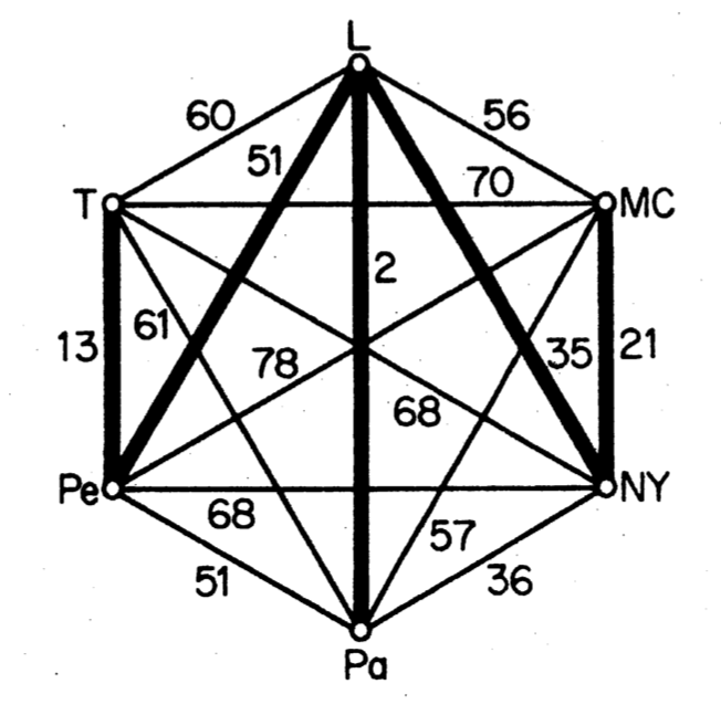
On the left side, the initial network. On the right side, a solution to this problem, with a cost of 12154.

Now, let’s load the data.

// Load data
String[] cities = new String[]{
  "London", "Mexico City", "New York", "Paris", "Peking", "Tokyo"
};

int[][] distances = 
{
  {0, 5558, 3469, 214, 5074, 5959},   // L
  {5558, 0, 2090, 5725, 7753, 7035},  // MC
  {3469, 2090, 0, 3636, 6844, 6757},  // NY
  {214, 5725, 3636, 0, 5120, 6053},   // Pa
  {5074, 7753, 6844, 5120, 0, 1307},  // Pe
  {5959, 7035, 6757, 6053, 1307, 0},  // T
}

Imports and model

Before going further, create a class and import the following classes.

import org.chocosolver.solver.Model;
import org.chocosolver.solver.Solver;
import org.chocosolver.solver.variables.IntVar;
import org.chocosolver.util.objects.graphs.UndirectedGraph;
import org.chocosolver.util.objects.setDataStructures.SetType;
import org.chocosolver.solver.variables.UndirectedGraphVar;

Then declare a model to work with in a method.

Model cop = new Model("The Connector Problem");

How to build GraphVar

There are 6 nodes in this complete graph. We can declare a GraphVar as an undirected graph, that is based on a lower bound which defines the mandatory elements (vertices and edges) and an upper bound which defines the optional elements. Elements can be removed from the upper bound or enforced in the lower bound. A GraphVar is considered as instantiated when the lower bound and the upper bound are equal.

UndirectedGraph GLB = new UndirectedGraph(cop, cities.length, SetType.BITSET, true);
UndirectedGraph GUB = new UndirectedGraph(cop, cities.length, SetType.BITSET, true);

The last parameter states that all nodes always remain in the graph. The nodes are labeled from 0 to cities.length-1. The lower bound of the GraphVar contains the cities but no edges since none of them are mandatory. The upper bound only contains the cities and the optional edges must now be declared.

for(int i = 0; i < cities.length; i++){
  for(int j = i+1; j < cities.length; j++){
      GUB.addEdge(i, j);   
  }  
}

It is now possible to declare the graph variable G as follow.

UndirectedGraphVar graph = cop.graphVar("G", GLB, GUB);

We can see how the current value of the domain of $G$:

private void printGLB(){
  System.out.println("Lower bound of G:");
  for (int n : graph.getMandatoryNodes()) {
      System.out.printf("\t%s -> {", cities[n]);
      for (int v : graph.getMandatoryNeighborsOf(n)){
          System.out.printf("%s, ", cities[v]);
      }
      System.out.print("}\n");
  }
}
 
private void printGUB(){ 
  System.out.println("Upper bound of G:");
    for (int n : graph.getPotentialNodes()) {
      System.out.printf("\t%s -> {", cities[n]);
      for (int v : graph.getPotentialNeighborsOf(n)){
          System.out.printf("%s, ", cities[v]);
      }
      System.out.print("}\n");
  }
}

Calling these two methods prints

Lower bound of G:
  London -> {}
  Mexico City -> {}
  New York -> {}
  Paris -> {}
  Peking -> {}
  Tokyo -> {}
Upper bound of G:
  London -> {Mexico City, New York, Paris, Peking, Tokyo, }
  Mexico City -> {London, New York, Paris, Peking, Tokyo, }
  New York -> {London, Mexico City, Paris, Peking, Tokyo, }
  Paris -> {London, Mexico City, New York, Peking, Tokyo, }
  Peking -> {London, Mexico City, New York, Paris, Tokyo, }
  Tokyo -> {London, Mexico City, New York, Paris, Peking, }

Constraints

In order to impose that G is a spanning tree, we post a degree constrained-minimum spanning tree (or dcmst). Since this constraint offers to constraint the degrees too, it is required to declare variables that define the degree of each node. This is achieved through a channeling constraint between G and IntVars.

IntVar[] degrees = cop.intVarArray("degree", cities.length, 0, cities.length-1);
cop.degrees(graph, degrees).post();

Note that the constraint is posted to the model. Actually, the other option would be to reify it.

We also need to get the cost of the spanning tree, in order to minimize it.

IntVar totalCost = cop.intVar("cost", 0, 6*99_999);

Now everything is up to post the constraint that ensure that G is a minimum spanning tree:

cop.dcmst(graph,degrees,totalCost,distances,0).post();

Objective and solving

Since we deal with a Constraint Optimization Problem, an objective variable has to be declared, together with the policy:

cop.setObjective(Model.MINIMIZE, totalCost);

And we are ready to run the resolution:

Solver slv = cop.getSolver();
slv.showShortStatistics();
//slv.reset();
while (slv.solve()){
    System.out.printf("Spanning tree of cost %d\n", totalCost.getValue());
    printGLB();
}

which prints :

...
Model[The Connector Problem], 13 Solutions, MINIMIZE cost = 12154, Resolution time 0.389s, Time to best solution 0.389s, 612 Nodes (1,573.0 n/s), 1184 Backtracks, 0 Backjumps, 583 Fails, 0 Restarts
Spanning tree of cost 12154
Lower bound of G:
  London -> {New York, Paris, Peking, }
  Mexico City -> {New York, }
  New York -> {London, Mexico City, }
  Paris -> {London, }
  Peking -> {London, Tokyo, }
  Tokyo -> {Peking, }
Model[The Connector Problem], 13 Solutions, MINIMIZE cost = 12154, Resolution time 0.416s, Time to best solution 0.389s, 704 Nodes (1,692.0 n/s), 1383 Backtracks, 0 Backjumps, 679 Fails, 0 Restarts

A better search strategy

It is possible to give the solver hints to better explore the search space. This is done by defining a search strategy. In our case, we want to select first edges associated to small distance.

import org.chocosolver.solver.search.strategy.strategy.GraphCostBasedSearch;
// ...


slv.reset(); // required to run the resolution twice
GraphCostBasedSearch mainSearch = new GraphCostBasedSearch(graph, distances);
mainSearch.configure(GraphCostBasedSearch.MIN_COST);
slv.setSearch(mainSearch);
while (slv.solve()){
    System.out.printf("Spanning tree of cost %d\n", totalCost.getValue());
    printGLB();
}

which results in:

Model[The Connector Problem], 1 Solutions, MINIMIZE cost = 12154, Resolution time 0.002s, Time to best solution 0.002s, 6 Nodes (2,717.0 n/s), 0 Backtracks, 0 Backjumps, 0 Fails, 0 Restarts
Spanning tree of cost 12154
Lower bound of G:
  London -> {New York, Paris, Peking, }
  Mexico City -> {New York, }
  New York -> {London, Mexico City, }
  Paris -> {London, }
  Peking -> {London, Tokyo, }
  Tokyo -> {Peking, }
Model[The Connector Problem], 1 Solutions, MINIMIZE cost = 12154, Resolution time 0.077s, Time to best solution 0.002s, 506 Nodes (6,532.8 n/s), 1011 Backtracks, 0 Backjumps, 505 Fails, 0 Restarts

The entire code

String[] cities = new String[]{
  "London", "Mexico City", "New York", "Paris", "Peking", "Tokyo"
};

int[][] distances = 
{
  {0, 5558, 3469, 214, 5074, 5959},   // L
  {5558, 0, 2090, 5725, 7753, 7035},  // MC
  {3469, 2090, 0, 3636, 6844, 6757},  // NY
  {214, 5725, 3636, 0, 5120, 6053},   // Pa
  {5074, 7753, 6844, 5120, 0, 1307},  // Pe
  {5959, 7035, 6757, 6053, 1307, 0},  // T
};


Model cop = new Model("The Connector Problem");

UndirectedGraph GLB = new UndirectedGraph(cop, cities.length, SetType.BITSET, true);
UndirectedGraph GUB = new UndirectedGraph(cop, cities.length, SetType.BITSET, true);
for(int i = 0; i < cities.length; i++){
  for(int j = i+1; j < cities.length; j++){
      GUB.addEdge(i, j);   
  }  
}
UndirectedGraphVar graph = cop.graphVar("G", GLB, GUB);

IntVar[] degrees = cop.intVarArray("degree", cities.length, 0, 2);
cop.degrees(graph, degrees).post();

IntVar totalCost = cop.intVar("cost", 0, 6*99_999);
cop.setObjective(Model.MINIMIZE, totalCost);

cop.dcmst(graph,degrees,totalCost,distances,0).post();

Solver slv = cop.getSolver();

GraphCostBasedSearch mainSearch = new GraphCostBasedSearch(graph, distances);
mainSearch.configure(GraphCostBasedSearch.MIN_COST);
slv.setSearch(mainSearch);

slv.showShortStatistics();
while (slv.solve()){
    System.out.printf("Spanning tree of cost %d\n", totalCost.getValue());
    printGLB();
}